
Editorial
This problem can be solved by utilizing the solutions from problems B2 and B6.
The quantum circuit diagram for the case where is shown as follows
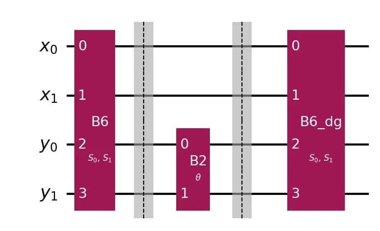 ,
where B6 and B2 in the quantum circuit diagram represent the quantum circuits from the solutions to problems B6 and B2, respectively. The notation B6_dg represents the inverse operation of B6.
Let's walk through the state transitions.
First, we apply the quantum phase estimation quantum circuit, which is the solution to problem B6.
Next, we apply the oracle, which is the solution to problem B2.
Finally, we apply the inverse operation of the quantum phase estimation quantum circuit, which is the solution to problem B6.
The quantum circuit depth is .
Sample Code
Below is a sample program:
import math

from qiskit import QuantumCircuit, QuantumRegister


def phase_estimation(n: int, m: int, S: list[int]) -> QuantumCircuit:
    def qft(n: int) -> QuantumCircuit:
        qc = QuantumCircuit(n)

        for i in reversed(range(n)):
            qc.h(i)
            for j in reversed(range(i)):
                qc.cp(math.pi / 2 ** (i - j), j, i)

        for i in range(n // 2):
            qc.swap(i, n - i - 1)

        return qc

    x, y = QuantumRegister(n), QuantumRegister(m)
    qc = QuantumCircuit(x, y)

    qc.h(y)

    for j in range(m):
        for i in range(n):
            theta = (2 * math.pi * S[i] / 2**m) * 2**j
            qc.cp(theta, x[i], y[j])

    qc.compose(qft(m).inverse(), y, inplace=True)

    return qc


def rotation_L(n: int, L: int, theta: float) -> QuantumCircuit:
    qc = QuantumCircuit(n)

    for i in range(n):
        if not (1 << i) & L:
            qc.x(i)

    if n == 1:
        qc.p(theta, n - 1)
    else:
        qc.mcp(theta, list(range(n - 1)), n - 1)

    for i in range(n):
        if not (1 << i) & L:
            qc.x(i)

    return qc


def solve(n: int, m: int, L: int, S: list[int], theta: float) -> QuantumCircuit:
    x, y = QuantumRegister(n), QuantumRegister(m)
    qc = QuantumCircuit(x, y)

    oracle = phase_estimation(n, m, S)

    qc.compose(oracle, inplace=True)
    qc.compose(rotation_L(m, L, theta), y, inplace=True)
    qc.compose(oracle.inverse(), inplace=True)

    return qc